Tidy Tuesday: Australian Frogs

This week’s data is from the FrogID dataset, which I sourced and curated! The dataset contains 6 years worth of frog recordings. To meet file size requirements, I limited the Tidy Tuesday dataset to just 2023 data.

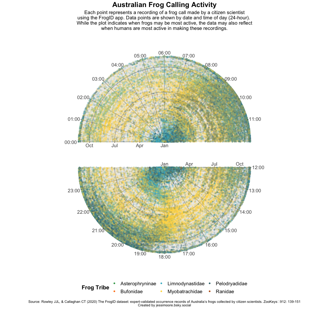
I made a relatively quick plot this week to try to bump up my efficiency. Not a lot of info can be gleaned from the tribe colours, apart from that Pelodryadidae (Treefrogs) appear to be the most common, followed by Myobatrachidae (Ground/water frogs). The seasonal and time-of-day patterns are interesting and to be expected, although I wonder how much these are influenced by when people are most likely to be outside and recording frogs.

library(tidyverse)
library(patchwork)
library(paletteer)

tuesdata <- tidytuesdayR::tt_load(2025, week = 35)

frogID_data <- tuesdata$frogID_data
frog_names <- tuesdata$frog_names

frog_names[frog_names == '—'] <- NA

frogs <- frogID_data %>%
  left_join(frog_names, by = "scientificName") %>%
  select(c(scientificName, eventDate, eventTime, commonName, stateProvince,
           decimalLatitude, decimalLongitude, tribe)) %>%
  drop_na(commonName)

frogs_am <- frogs %>%
  filter(eventTime < hms("12:00:00"))

frogs_pm <- frogs %>%
  filter(eventTime >= hms("12:00:00"))

am <- ggplot(frogs_am, aes(eventTime, eventDate, color = tribe)) +
    geom_point(alpha = 0.15) +
    scale_x_time(breaks = seq(0, 23 * 3600, by = 3600),
                 labels = function(x) strftime(x, "%H:%M")) +
    scale_color_paletteer_d("ggthemes::Classic_Green_Orange_6") +
    coord_radial(expand = FALSE, r.axis.inside = TRUE,
                 start = -0.5*pi, end = 0.5*pi) +
    guides(color = guide_legend(override.aes = list(alpha = 1))) +
    labs(x = NULL, y = NULL, color = "Frog Tribe")

pm <- ggplot(frogs_pm, aes(eventTime, eventDate, color = tribe)) +
    geom_point(alpha = 0.15) +
    scale_x_time(breaks = seq(0, 23 * 3600, by = 3600),
                 labels = function(x) strftime(x, "%H:%M")) +
    scale_color_paletteer_d("ggthemes::Classic_Green_Orange_6") +
    coord_radial(expand = FALSE, r.axis.inside = TRUE,
                 start = 0.5*pi, end = -0.5*pi) +
    guides(color = guide_legend(override.aes = list(alpha = 1))) +
    labs(x = NULL, y = NULL, color = "Frog Tribe")


combined_plot <- am / pm + plot_layout(guides = "collect") +
  plot_annotation(
    title = "Australian Frog Calling Activity",
    subtitle = glue::glue("Each point represents a recording of a frog call made by a citizen scientist
                           using the FrogID app. Data points are shown by date and time of day (24-hour). 
                           While the plot indicates when frogs may be most active, the data may also reflect
                           when humans are most active in making these recordings."),
    caption = glue::glue("Source: Rowley JJL, & Callaghan CT (2020) The FrogID dataset: expert-validated occurrence records of Australia’s frogs collected by citizen scientists. ZooKeys 912: 139-151
                         Created by jessimoore.bsky.social")
    ) &
  theme(axis.text = element_text(size = 14),
          panel.grid.major = element_line(color = "grey25", linewidth = 0.3),
          legend.key = element_blank(),
        plot.title = element_text(size = 20, face = "bold", hjust = 0.5),
        plot.subtitle = element_text(size = 14, hjust = 0.5),
        legend.title = element_text(size = 16, face = "bold"),
        legend.text = element_text(size = 14),
        legend.position = "bottom",
        plot.caption = element_text(size = 10, hjust = 0.5),
        plot.caption.position = "plot")