Tidy Tuesday: Billboard Hot 100 #1s

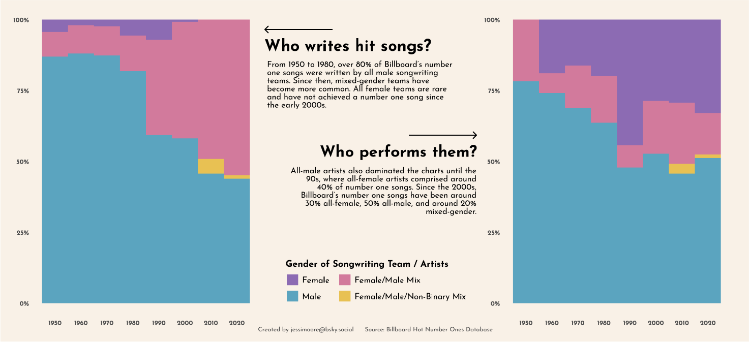
This week’s TT dataset came from Billboard Hot 100 Number Ones Database. With such a rich dataset and so many variables it was difficult to know where to even begin. I tried out a few options before settling on exploring gender of songwriters and artists over time.

I edited the final combined plot using Figma, which made customising the text much easier.

Code

library(tidyverse)
library(patchwork)
library(paletteer)
library(ggstream)
library(sysfonts)
library(showtext)

tuesdata <- tidytuesdayR::tt_load('2025-08-26')
billboard <- tuesdata$billboard %>% 
  drop_na(songwriter_male)

b <- billboard %>%
  mutate(year = 10 * (year(as.Date(date)) %/% 10),
         songwriter_male = factor(case_when(
           songwriter_male == 0 ~ "Female",
           songwriter_male == 1 ~ "Male",
           songwriter_male == 2 ~ "Female/Male Mix",
           songwriter_male ==3 ~ "Female/Male/Non-Binary Mix"))) %>%
  # removing 2025 as there is only one song in dataset
  filter(year != 2025) %>%
  count(year, songwriter_male)

pal <- c("#8C6BB3", "#D27A9C", "#E8C153", "#5BA4BF")
bg <- "#F4F4ED"
font_add_google("Josefin sans", "josefin")
ft <- "josefin"
showtext_auto()

theme <- theme(panel.grid = element_blank(),
        plot.background = element_rect(fill = bg, color = bg))

p <- ggplot(b,
            aes(year, n, fill = songwriter_male))+
  geom_col(position = "fill", width = 10) +
  scale_y_continuous(labels = scales::percent) +
  scale_fill_manual(values = pal) +
  scale_x_continuous(
    breaks = seq(1950,2020, 
                 by = 10)) +
  labs(x = NULL, y = NULL, fill = "Gender of Songwriting Team") +
  theme_minimal() +
    theme(axis.text = element_text(family = ft, size = 12, face = "bold"),
        legend.title = element_text(family = ft, size = 12, face = "bold"),
        legend.text = element_text(family = ft, size = 12)) +
  theme

b2 <- billboard %>%
  mutate(year = 10 * (year(as.Date(date)) %/% 10),
         artist_male = factor(case_when(
           artist_male == 0 ~ "Female",
           artist_male == 1 ~ "Male",
           artist_male == 2 ~ "Female/Male Mix",
           artist_male ==3 ~ "Female/Male/Non-Binary Mix"))) %>%
  # removing 2025 as there is only one song in dataset
  filter(year != 2025) %>%
  count(year, artist_male)

p2 <- ggplot(b2,
            aes(year, n, fill = artist_male))+
  geom_col(position = "fill", width = 10) +
  scale_y_continuous(labels = scales::percent) +
  scale_x_continuous(
    breaks = seq(1950, 2020,
                 by = 10)) +
  scale_fill_manual(values = pal) +
  labs(x = NULL, y = NULL, fill = "Gender of Songwriting Team") +
  theme_minimal() +
    theme(axis.text = element_text(family = ft, size = 12, face = "bold"),
        legend.title = element_text(family = ft, size = 12, face = "bold"),
        legend.text = element_text(family = ft, size = 12)) +
  theme

# Create the titles
t1 <- 
  ggplot() +
  theme_void() +
  geom_text(aes(x = 0, y = 0), label = "Who writes hit songs?", family = ft, size = 8, lineheight = .5, fontface = 'bold') +
  theme(axis.text = element_blank())

t2 <- 
  ggplot() +
  theme_void() +
  geom_text(aes(x = 0, y = 0), label = "Who performs them?", family = ft, size = 8, lineheight = .5, fontface = 'bold')  +
  theme(axis.text = element_blank())

# Design patchwork layout
layout <- c(
  area(1,1,3,1), #p1
  area(1,2,1,2), #t1
  area(2,2,2,2), #legend
  area(3,2,3,2), #t2
  area(1,3,3,3) #p2
)

combined_plot <- p + t1 + guide_area() + t2 + p2 + 
  plot_layout(design = layout, guides = "collect") &
  theme